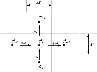
Figure 3.5.1 Node layout for computing solute flux
| [TOC] | 3.5 Estimating Fluxes for Advection and Dispersion | [Prev. Page] | [Next Page] |
Figure 3.5.1 illustrates the spatial layout of nodes and notation used by this section to describe how the model calculates advection and dispersion.
Figure 3.5.1 Node layout for computing solute flux
In the above figure, x-1 refers to the upstream node in the X direction, x+1 refers to the downstream node in the X direction. The same applies in the Y direction. C and q refer to the concentration of the kth species and the specific discharge across element boundaries, respectively.
The continuity equation calculates the change in concentration due to flux, D Cfk, by drawing a control volume around the center node:
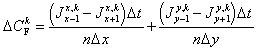 |
(3.7) |
Where: D CFk = change in concentration of kth species due to advection-dispersion = flux of solute k from node x-1 to center node
n = element porosity D t = time step D X = grid spacing in x direction D Y = grid spacing in y direction
The MCS method (Poulsen, 1994) is used to compute the flux between two nodes. It is an explicit finite difference method corrected for numerical dispersion. Equation (3.8) gives the equation used to calculate the flux between the two nodes. See Appendix C for a detailed discussion of the MCS method.
| (3.8) |
Where: = specific discharge from node x-1 to node center node
= mass flux from node x-1 to center node
Ckx = concentration of kth species in node x Ckx-1 = concentration of kth species in node x-1 D t = timestep n = porosity Dx = dispersion in X direction D x = node spacing in X direction Dxy = cross dispersion coefficient
| [Home] | [Table of Contents] | [Prev. Page] | [Next Page] |
| A Two Dimensional Numerical Model for Simulating the
Movement and Biodegradation of Contaminants in a Saturated Aquifer © Copyright 1996, Jason E. Fabritz. All Rights Reserved. |
|||