This appendix describes how the equation for the optimal timestep was developed. It describes the theory behind the criteria, as well as the calculations made to arrive at the equations. Calculations for one and two dimensions are included.

The method used to determine the maximum allowable timestep was first used by Wind and van Doorne (1975) to calculate criteria used in solving the variably saturated flow problem using the MCS method. The equations used in the study were quite similar in structure to the governing equations here. The method is repeated here.

The timestep criteria sought in this appendix is based on the theory of "amplification" of roundoff errors. Due to machine precision, there will always be some small error in the calculations. It is desired to determine the timestep at which these errors will not "amplify" or cause larger errors in subsequent time intervals. If the timestep is too large, the error, originally introduced by roundoff, will be a factor larger in the subsequent time step. The same error will then be another factor larger in the following time step and so on. This will lead to oscillations in space as iterations progress, and may even cause the method to fail.

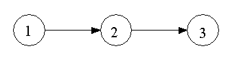
Since it is far easier to explain the mathematics for a one dimensional aquifer, the one dimensional case is presented first. Consider the case of the following node segments in one dimension:

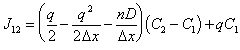
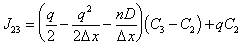
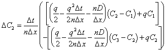
From the MCS method, the fluxes into node 2 and out of node 2 respectively are:

	(E.1)
	(E.2)

Where:	q = darcy flux in the x direction (a positive value)
	D x = distance between nodes
	n = material porosity
	D = dispersion coefficient
	C1 = solute concentration in node 1
	C2 = solute concentration in node 2
	C3 = solute concentration in node 3

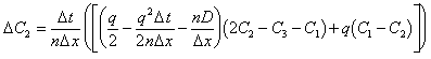
Now, over a timestep, D t, the change in concentration at node two can be given as:

(E.3)

or when combined with equations (E.1) and (E.2) can be given as:

	(E.4)
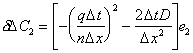
	(E.5)

Equation (E.5) is the "correct" change in concentration at node two over the time interval D t Now introduce a small error, e₂, such that the calculation of C₂ at the beginning of the timestep is in error:

(E.6)

Denoting the change in concentration using the "incorrect" value for C₂ as D C₂^*, the error in the change of concentration over D t can be computed:

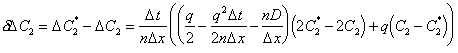(E.7)

or:

(E.8)

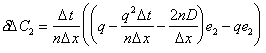
Simplifying:

(E.9)

Dividing by the error:

(E.10)

Where Co is the courant number and Pe is the peclet number.

In order to keep errors from "amplifying", the magnitude of the error produced by Equation (E.5) must be less than the original error. In mathematical terms this can be stated:

(E.11)

Which translates into:

(E.12)

and

(E.13)

Equation (E.12) is satisfied for all Pe > 0 and Co> 0. However Equation (E.13) is not. The solution is:

(E.14)

Equation (E.14) must be satisfied at all nodes in the simulation in order to prevent errors from amplifying. The easiest way to satisfy (E.14) is to adjust the global timestep. The equation used to calculate the maximum timestep can be derived from Equation (E.14) to be:

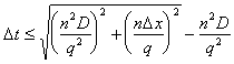(E.15)

In addition to the maximum allowable timestep, numerical analysis showed there exists a minimum allowable timestep as well. The error caused by too small of a timestep is only a fraction of the error caused by too large of a timestep. However, the error is too large to ignore.

Consider a special case of the one dimensional example above. In the case of a retreating solute front, d C/d x > 0, d C/d t < 0, q > 0, the flux out of a node over a timestep must not be greater than the solute concentration in that node. Or in other words, the flux cannot be so great that it will cause the concentration at the end of the timestep to become negative. In mathematical terms this can be stated.

(E.16)

Since in this case, (C₂-C₁) is positive, it can be demonstrated the following equation must be satisfied:

(E.17)

Rearranging yields:

	(E.18)
	(E.19)

Which translates into a minimum timestep criteria:

(E.20)

or a courant number criteria:

(E.21)

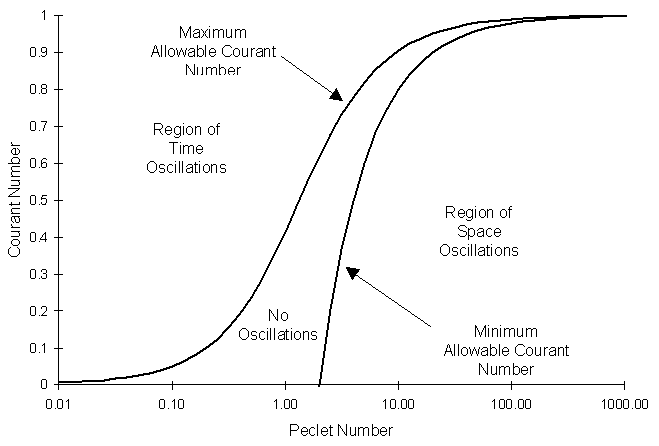
The following graph illustrates the different timestep criteria equations for a one dimensional aquifer as a function of peclet and courant numbers superimposed with contour lines of the RSSE. For a detailed discussion of the RSSE, see the main text.

Equations (E.18) and (E.21) are only for one dimension. It is necessary to repeat the analysis for two dimensions. Consider the case of the following node segments in two dimensions:

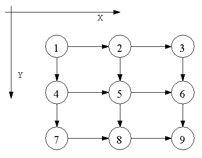
From the MCS method, the fluxes into and out of node 5 are:

	(E.22)
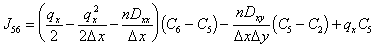	(E.23)
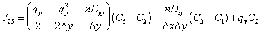	(E.24)
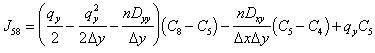	(E.25)

Over the timestep, D t, the change in concentration at node five can be given as:

(E.26)

Simplifying Equations (E.22) to (E.26) yields:

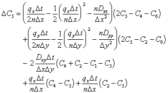(E.27)

The associated error in the change in concentration is:

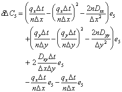(E.28)

And the relative error becomes:

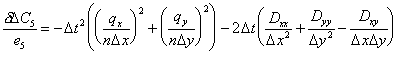(E.29)

The associated inequality is:

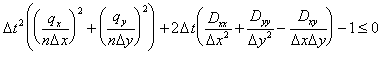(E.30)

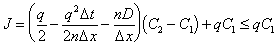
Therefore the maximum timestep for a two-dimensional simulation that allows stability is:

(E.31)

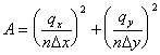
Where:

In addition, the corresponding minimum timestep criteria in two dimensions was developed using the similarity of the other one and two-dimensional criteria equations:

(E.32)

It can be shown, in the case of one-dimension, the above two dimensional equations reduce to the one dimensional equations calculated above.