This section evaluates model performance in simulating kinetic reactions. The tests do not include advection and dispersion. The aquifer systems in this section are similar to what one would expect under completely mixed conditions.

This section presents two figures for each type of kinetic reaction. The first figure illustrates model solution as a function of time compared to the true solution. The second figure plots RSSE (for one node) as a function of calculation time step. The calculation timestep is analogous to the timestep used to compute advection and dispersion fluxes. Some of the kinetic systems evaluated in this section are highly non-linear and require numerical methods to solve. The "true" solution used in these tests is calculated using the Mathematicaä software package (Wolfram Research Inc., 1988). The initial conditions in both figures are the same.

The following tests represent a small subset of the possible combinations of input parameters. It is not possible to anticipate all combinations and systems possible. The examples in this section include first order decay and competitive Monod reactions. Appendix F contains additional examples.

The equation representing first order decay is:

(4.9)

Where:	d C/d t = time rate of change of concentration (M/L3·T)
	C = concentration of solute species (M/L3)
	k = decay coefficient (T-1)

Figure 4.8.1 illustrates the model solution compared to the true solution using a calculation timestep of 2.0 and varying decay coefficients. Symbols and lines represent numerical and true values, respectively.

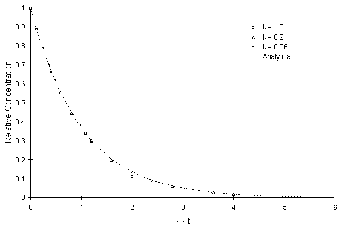
Figure 4.8.1 First Order Decay with Varying k.

Figure 4.8.2 illustrates the numerical solution errors at the time step of 20.0 for various decay coefficients.

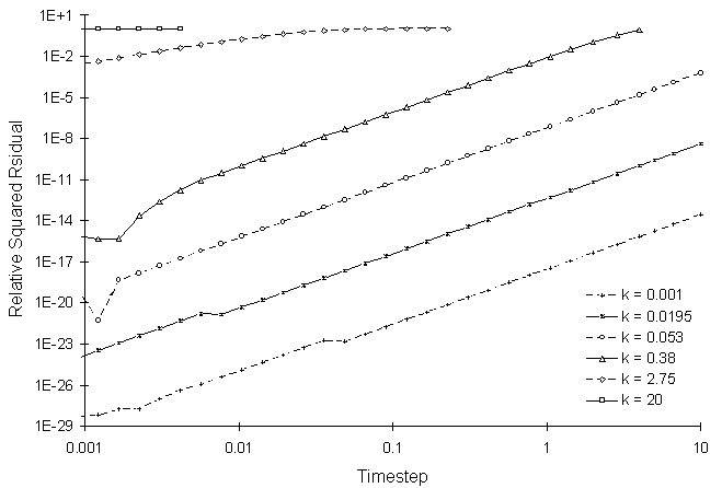
Figure 4.8.2 RSSE as a Function of First Order Decay Coefficient and Calculation Timestep

Figure 4.8.2 shows that increasing the rate coefficient and timestep increases the simulation RSSE value.

A simplified version of the competitive inhibition equation is:

	(4.10)
	(4.11)

Where:	Ca = concentration of electron acceptor (M/L3)
	Cd = concentration of electron donor (M/L3)
	Ci = concentration of inhibitor (M/L3)
	X = biomass concentration (M/L3)
	k = maximum rate constant (L6/M3·T)
	Ksa = half saturation constant for electron acceptor (M/L3)
	Ksd = half saturation constant for electron donor (M/L3)
	Ya = stoichiometry coefficient for electron acceptor
	Yd = stoichiometry coefficient for electron donor
	Yx = stoichiometry coefficient for biomass
	Yi = stoichiometry coefficient inhibitor

Figure 4.8.3 compares the model and true solutions using a global calculation timestep of 2.0. For this test k = 0.2, K_sa = 5.0, K_sd = 10.0, Y_x = 0.5, Y_A = 1.0, Y_D = 2.5 and Y_i = 0.2. Circles and lines denote numerical and true values, respectively.

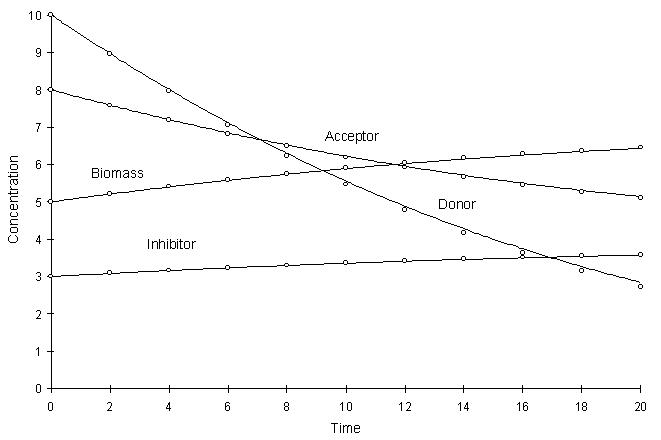
Figure 4.8.3 Competitive Monod Decay k = 0.2, K_sa = 5.0, K_sd = 10.0, Y_x = 0.5, Y_A = 1.0, Y_D = 2.5, _Yi = 0.2.

Figure 4.8.4 illustrates the Relative Squared Residual as a function of calculation time step:

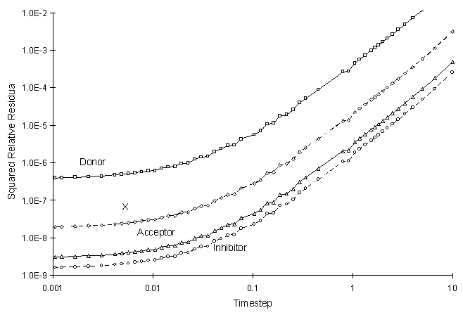
Figure 4.8.4 Squared Relative Residual as a Function of Global Timestep for Competitive Monod Decay.

See Appendix F for analysis of other kinetic reactions.