User's Manual, - 13.2 Lesson 2, Kinetic Sorption and Desorption

13.2 Lesson 2, Kinetic Sorption and Desorption

This lesson will demonstrate how to add a partitioning reaction to a simulation. This lesson uses the simulation created in Lesson One. If the simulation in lesson one is still open, close all windows and save it. If it is not open, then open it with the Open command from the file menu.

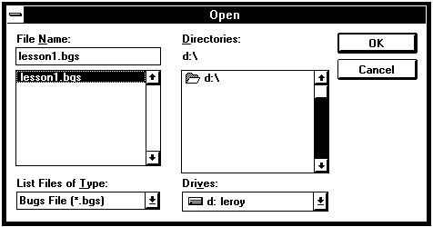
First, save the simulation under another name. From the File menu, select Save As. In the save as dialog box enter any appropriate name, for example "Lesson2".

It is necessary to add a parameter to the simulation to represent the sorbed phase of O2. From the Windows menu, select Parameters.

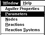
Click the Add button and enter "O2 (s)" as the name of the new parameter (sorbed species.)

This is an immobile (sorbed) parameter, therefore all the default values are adequate. Close the Parameters window. From the Windows menu, select Reactions.

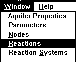
Next we’ll add a reaction representing the partitioning of the solute and sorbed phase (partitioning "O2" and "O2 (s)"). Click on the Add Button and enter "O2 Partitioning" as the name of the reaction.

This reaction will be a kinetic linear isotherm partitioning reaction. Bring up the Type screen by clicking on the Type tab if necessary.

Select Linear under the Kinetic Sorption reaction type.

Next we’ll add the rate data for the partitioning reaction. Select the Rate tab.

The rate data will appear. The linear driving force will be a one to one ratio between "O2" and "O2 (s)". Enter values so that they match the following example.

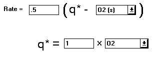
Now that the rate data is entered, enter the Stoichiometry data. Click on the Stoichiometry tab.

The solute, O2, will be moving to the Sorbed phase, O2 (s), when the rate is positive. For O2 enter -1.0. For O2 (s) enter 1.0.

BUGS will then display the Stoichiometry reaction.

Next, add this reaction to the entire aquifer system. Click on the Systems tab.

To include this reaction in all of the reaction systems, click on the include all button, this includes the reaction in both the "Boundary Condition" reaction system and "Interior" reactions system.

Now this reaction will be included both in the boundary condition reaction system and the interior reaction system.

Close the reactions window. Save the simulation data before running the simulation. A shortcut way of saving a simulation is to click the Save button on the tool bar.

Run the simulation, chose Simulate from the Run Menu

The screen will appear similar to the following.

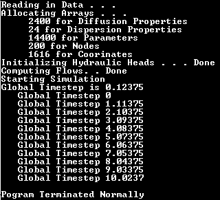
To view the profile output select Profile Graph from the Windows menu. From the Parameters menu ensure O2 and O2 (s) are checked. Move the time period to 7. The graph should appear to be similar to the following.

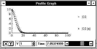
Notice, the O2 (s) front lags behind the O2 Solute front, as it should with kinetic sorption.

This concludes kinetic sorption and desorption tutorial, if you have any questions please feel free to contact us at jasonf@bugbytes.com.

� Copyright 1998, BUGBYTES, Inc. All Rights Reserved. BUGBYTES, BUGS and the Bug logo are trademarks of BUGBYTES, Inc. All other product names are trademarks, registered trademarks, or service marks of their respective owners.

Last Updated October 1, 2001