This work uses the MCS solution scheme developed by Wind and van Doorne (1975), and Poulsen (1994) to solve the advection-dispersion portion of the system of equations. This appendix is a quick overview of the calculations used to derive the equations.

First, consider advection and dispersion in a one dimensional aquifer. The fundamental equation for the change in concentration of a solute in time in one-dimensional space is:

(C.1)

Where:	d C/d t = time rate of change in concentration
	C = concentration
	D = dispersion coefficient
	q = darcy flux
	n = material porosity
	R = net rate of reaction (sink/source term)

For this discussion we are only interested in the advection-dispersion part of equation (C.1), the reactive portion will be ignored. Equation (C.1) can therefore be rewritten in the form:

(C.2)

Where J is the equation of solute flux in the x direction. The solute flux equation is defined as:

(C.3)

The above equation is the one of interest. Next, it will be necessary to convert equation (C.3) into a discretized form. This will be done by setting boundary conditions and integrating equation (C.3) with respect to space at a given time instant. Rewriting equation (C.3) in standard form for the solution of the first order linear differential equation yields:

(C.4)

The next step is to solve the homogeneous equation. D and q are assumed to be constant and uniform over the area of integration.

	(C.5)
	(C.6)

Next, the solution of the non-homogeneous equation is computed. K’(x) refers to the derivative of the constant of integration, K, with respect to x.

	(C.7)
	(C.8)
	(C.9)
	(C.10)

Therefore:

	(C.11)
	(C.12)

To eliminate the constant of integration "K, the boundary conditions (C=C₁,x=x₁) and (C=C₂,x=x₂) are substituted into equation (C.12):

(C.13)

With rearrangement yields:

(C.14)

J is the flux from boundary (1) to boundary (2). Equation (C.14) is prone to artificial numerical dispersion. It is necessary to define a term to correct the actual dispersion coefficient for this artificial numerical dispersion.

First, it is necessary to explain some nomenclature. t refers to the current time period, or the beginning of the current time interval. t+D t refers to the next time period, or the ending of the current time interval. x refers to the current index in the aquifer. x-D x refers to the previous index and x+D x to the next index. D t refers to the time interval. D x refers to the grid spacing.

The equation for change in concentration as a function of time can be written:

(C.15)

In discrete terms, it is written:

(C.16)

Expanding yields:

(C.17)

Equation (C.17) can be considered a finite-difference approximation to the advection-dispersion equation (Poulsen 1991). A Taylor expansion based method was used to find and correct for second order numerical errors. If the following Taylor expansion series are used (neglecting terms of fourth order and higher):

	(C.18)
	(C.19)
	(C.20)
	(C.21)

Rewriting equation (C.1) to solve for the change in concentration in time, then differentiating twice with respect to time:

	(C.22)
	(C.23)
	(C.24)

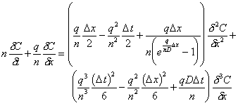
If equations (C.18) through (C.24) are substituted into equation (C.17) and simplified, the following equation will result:

(C.25)

When comparing equation (C.25) with equation (C.22), one can see the numerical correction. The second order term approximates the artificial numerical dispersion created by the numerical method. The numerical dispersion coefficient would be the difference between the second order term in equation (C.25) and the actual dispersion coefficient, or:

(C.26)

The next step is to determine how the correction for numerical dispersion fits into equation (C.14). First compare equation (C.14), which is the finite difference equation for flux between two nodes, with equation (C.3). Comparison of the terms in these equations which involve dispersion;

(C.27)

show that the "equivalent" dispersion term for the finite difference equation of solute flux is:

(C.28)

Equation (C.14) now becomes:

(C.29)

After inserting equations (C.26) and (C.28) into equation (C.29) and simplifying, the one dimensional equation for flux between two nodes in a one dimensional aquifer becomes:

(C.30)

It should be noted Equation (C.30) is also equivalent to the implementation of the FTBS mixing cell model used by Rao and Hathaway (1989) which cited the use of a numerical dispersion coefficient in the x direction to be:

(C.31)

Which is the same as calculated here, accounting for the difference in the conventions and placement of the porosity, n, and grid spacing, D x.

Equation (C.30) is only for one dimension. It is necessary to have an equation of flux which corresponds to a two dimensional aquifer. The fundamental equation for the change in conservative solute concentration as a function of time in two dimensions is:

(C.32)

Where:	Dxx =
	Dyy =
	Dxy =
	vx = pore water velocity in x direction, qx/n
	vy = pore water velocity in y direction, qy/n
	a l = longitudinal dispersivity
	a t = transverse dispersivity
	qz = darcy flux in x direction
	qy = darcy flux in y direction
	n = material porosity

Once again, from equation (C.32) the flux components in both the x and y directions respectively can be defined as:

	(C.33)
	(C.34)

It can be seen, there is an extra term, D_xy, included in the two dimensional flux equations. It is necessary to include this term in the FTBS solution scheme. For this discussion consider only the flux in the X direction (equation (C.33)), the equations for the Y direction will be similar.

Equation (C.33) can be re-written in the form:

(C.35)

Which is in the same form as the one dimensional flux equation. So, if the "effective" dispersion coefficient were to be defined as:

(C.36)

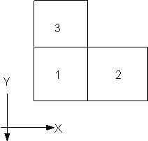
and using the following grid layout;

the discretized form would be:

(C.37)

Inserting equation (C.36) into (C.30) yields:

(C.38)

And when simplified:

(C.39)

Which is the equation for flux in the X direction between two nodes in a two dimensional aquifer. This is reasonable, since the numerical dispersion term is second order, not third. If one were to expect a correction for D_xy, it would have to be third order, which, in this implementation, was neglected.